---
title: "Animating Tracking Data"
output: rmarkdown::html_vignette
vignette: >
%\VignetteIndexEntry{Animating Tracking Data}
%\VignetteEngine{knitr::rmarkdown}
%\VignetteEncoding{UTF-8}
author: "Ross Drucker

 "
description: "Turning tracking coordinates into an animated play, combining
sportyR surfaces with gganimate."
opengraph:
image:
src: "https://raw.githubusercontent.com/sportsdataverse/sportyR/main/man/figures/sportyR_gh.png"
twitter:
card: summary_large_image
creator: "@sportyR_pkg"
---
```{r vignette-options, include = FALSE}
knitr::opts_chunk$set(
collapse = TRUE,
comment = "#>",
fig.path = "animating-tracking-data-",
out.width = "100%",
dpi = 600
)
options(rmarkdown.html_vignette.check_title = FALSE)
```
For the following vignette, you'll need the `sportyR`, `ggplot2`, and `gganimate` packages loaded into your workspace.
```{r setup}
library(sportyR)
library(ggplot2)
library(gganimate)
```
If this is your first experience with plotting tracking data, please check out the [plotting-tracking-data](plotting-tracking-data.html) vignette. Otherwise, let's see how to make GIFs with `sportyR` and `gganimate`.
## The Data
For this example, we'll use a play from Week 15 of the 2018 NFL season between the Chicago Bears and Green Bay Packers. Data made available for the [Big Data Bowl 2021](https://www.kaggle.com/c/nfl-big-data-bowl-2021) Kaggle competition.
```{r bdb-example-read-data}
# Load the play data
example_nfl_play <- data.table::fread(
glue::glue(
"https://raw.githubusercontent.com/sportsdataverse/sportyR/",
"main/data-raw/example-pbp-data.csv"
)
)
# Convert to data frame
example_nfl_play <- as.data.frame(example_nfl_play)
```
To keep things easy, let's specify the colors for each team's dots on the resulting GIF. We'll make the Bears [orange]{style="color: #c83803"} and the Packers [yellow]{style="color: #ffb612"}. The football will also need a dot to be seen; let's make it [brown]{style="color: #624a2e"}.
```{r bdb-example-prep-data}
# Prep data for plotting
example_nfl_play[example_nfl_play["team"] == "home", "color"] <- "#c83803"
example_nfl_play[example_nfl_play["team"] == "away", "color"] <- "#ffb612"
example_nfl_play[example_nfl_play["team"] == "football", "color"] <- "#624a2e"
```
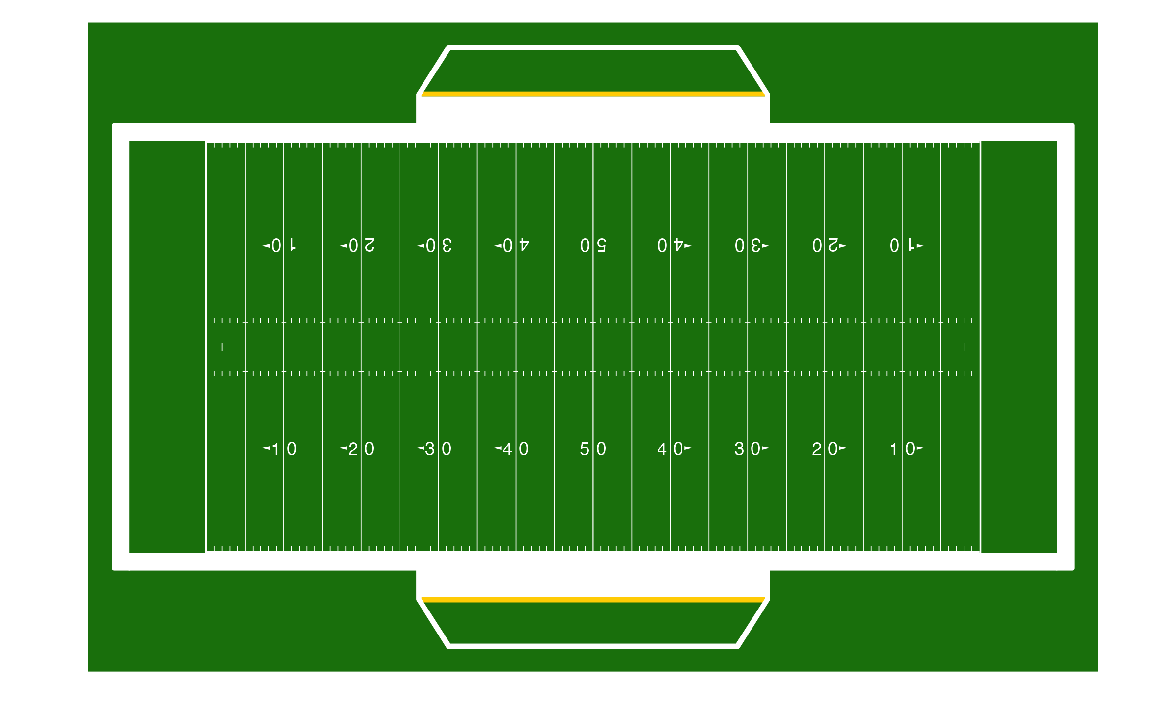
First, let's draw an NFL field via `geom_football("nfl")`. We'll adjust the origin to be in the lower left corner of the field, as per the notes on the coordinate system on the Kaggle page describing the data.
```{r bdb-example-draw-field, eval = FALSE}
# Create the field
nfl_field <- geom_football("nfl", x_trans = 60, y_trans = 26.6667)
# Display the field
nfl_field
```
{width=75%}
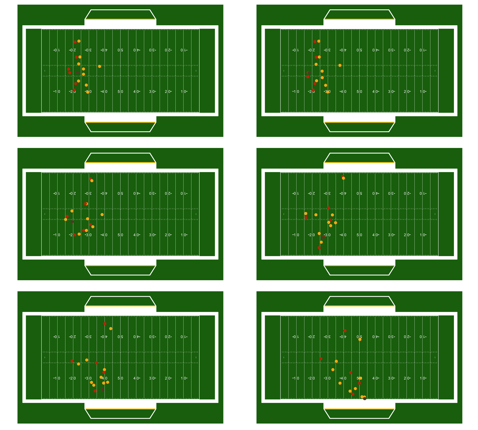
Looks good! Now, let's animate using `gganimate`.
```{r bdb-example-animate-play, eval = FALSE}
# Add the points on the field
play_anim <- nfl_field +
geom_point(
data = example_nfl_play,
aes(x, y),
color = example_nfl_play$color
) +
transition_time(example_nfl_play$frameId)
# Show the animation
play_anim
```
{width=75%}
Easy peasy. As noted on the [plotting-tracking-data](plotting-tracking-data.html) vignette, this too works so long as the geospatial data is provided and contains a way to identify and order the frames of the resulting GIF.
# **Our Authors**
- [Ross Drucker](https://x.com/rossdrucker9)
## **Citation**
To cite the [**`sportyR`**](https://sportyR.sportsdataverse.org/) R package in publications, use:
BibTeX Citation
```bibtex
@misc{sportyr,
author = {Ross Drucker},
title = {sportyR: Plot Scaled 'ggplot' Representations of Sports Playing Surfaces},
url = {https://sportyR.sportsdataverse.org/},
year = {2020}
}
```
## **Related SportsDataverse packages**
- [**cfbfastR**](https://cfbfastR.sportsdataverse.org/) - college football
- [**hoopR**](https://hoopR.sportsdataverse.org/) - men's basketball
- [**wehoop**](https://wehoop.sportsdataverse.org/) - women's basketball
- [**baseballr**](https://baseballr.sportsdataverse.org/) - baseball
- [**fastRhockey**](https://fastRhockey.sportsdataverse.org/) - hockey
- [**oddsapiR**](https://oddsapiR.sportsdataverse.org/) - betting odds
- [**sportyR**](https://sportyR.sportsdataverse.org/) - playing surfaces
- [**sportsdataverse-py**](https://py.sportsdataverse.org/) - the Python package
- [**sportsdataverse-R**](https://r.sportsdataverse.org/) - the R meta-package