---
title: "Getting started"
author: "Ewen Harrison"
output: rmarkdown::html_vignette
vignette: >
%\VignetteIndexEntry{Getting started}
%\VignetteEngine{knitr::rmarkdown}
%\VignetteEncoding{UTF-8}
---
```{r setup, include = FALSE}
knitr::opts_chunk$set(
collapse = TRUE,
comment = "#>"
)
```
The `finafit` package brings together the day-to-day functions we use to generate final results tables and plots when modelling.
I spent many years repeatedly manually copying results from R analyses and built these functions to automate our standard healthcare data workflow. It is particularly useful when undertaking a large study involving multiple different regression analyses. When combined with RMarkdown, the reporting becomes entirely automated. Its design follows Hadley Wickham's tidy tool manifesto.
## Installation and Documentation
Development lives on GitHub.
You can install the `finalfit` development version from CRAN with:
```{r eval=FALSE}
install.packages("finalfit")
```
It is recommended that this package is used together with dplyr, which is a dependent.
Some of the functions require `rstan` and `boot`. These have been left as `Suggests` rather than `Depends` to avoid unnecessary installation. If needed, they can be installed in the normal way:
```{r eval=FALSE}
install.packages("rstan")
install.packages("boot")
```
To install off-line (or in a Safe Haven), download the zip file and use `devtools::install_local()`.
## Main Features
### 1. Summarise variables/factors by a categorical variable
`summary_factorlist()` is a wrapper used to aggregate any number of explanatory variables by a single variable of interest. This is often "Table 1" of a published study. When categorical, the variable of interest can have a maximum of five levels. It uses `Hmisc::summary.formula()`.
```{r, warning=FALSE, message=FALSE}
library(finalfit)
library(dplyr)
# Load example dataset, modified version of survival::colon
data(colon_s)
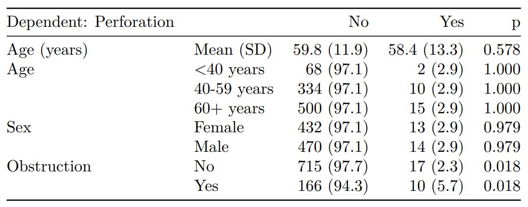
# Table 1 - Patient demographics by variable of interest ----
explanatory = c("age", "age.factor", "sex.factor", "obstruct.factor")
dependent = "perfor.factor" # Bowel perforation
colon_s %>%
summary_factorlist(dependent, explanatory,
p=TRUE, add_dependent_label=TRUE) -> t1
knitr::kable(t1, row.names=FALSE, align=c("l", "l", "r", "r", "r"))
```
When exported to PDF:
 See other options relating to inclusion of missing data, mean vs. median for continuous variables, column vs. row proportions, include a total column etc.
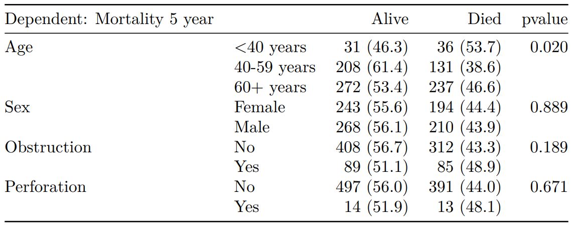
`summary_factorlist()` is also commonly used to summarise any number of variables by an outcome variable (say dead yes/no).
```{r, warning=FALSE, message=FALSE}
# Table 2 - 5 yr mortality ----
explanatory = c("age.factor", "sex.factor", "obstruct.factor")
dependent = 'mort_5yr'
colon_s %>%
summary_factorlist(dependent, explanatory,
p=TRUE, add_dependent_label=TRUE) -> t2
knitr::kable(t2, row.names=FALSE, align=c("l", "l", "r", "r", "r"))
```
See other options relating to inclusion of missing data, mean vs. median for continuous variables, column vs. row proportions, include a total column etc.
`summary_factorlist()` is also commonly used to summarise any number of variables by an outcome variable (say dead yes/no).
```{r, warning=FALSE, message=FALSE}
# Table 2 - 5 yr mortality ----
explanatory = c("age.factor", "sex.factor", "obstruct.factor")
dependent = 'mort_5yr'
colon_s %>%
summary_factorlist(dependent, explanatory,
p=TRUE, add_dependent_label=TRUE) -> t2
knitr::kable(t2, row.names=FALSE, align=c("l", "l", "r", "r", "r"))
```
 Tables can be knitted to PDF, Word or html documents. We do this in RStudio from a .Rmd document.
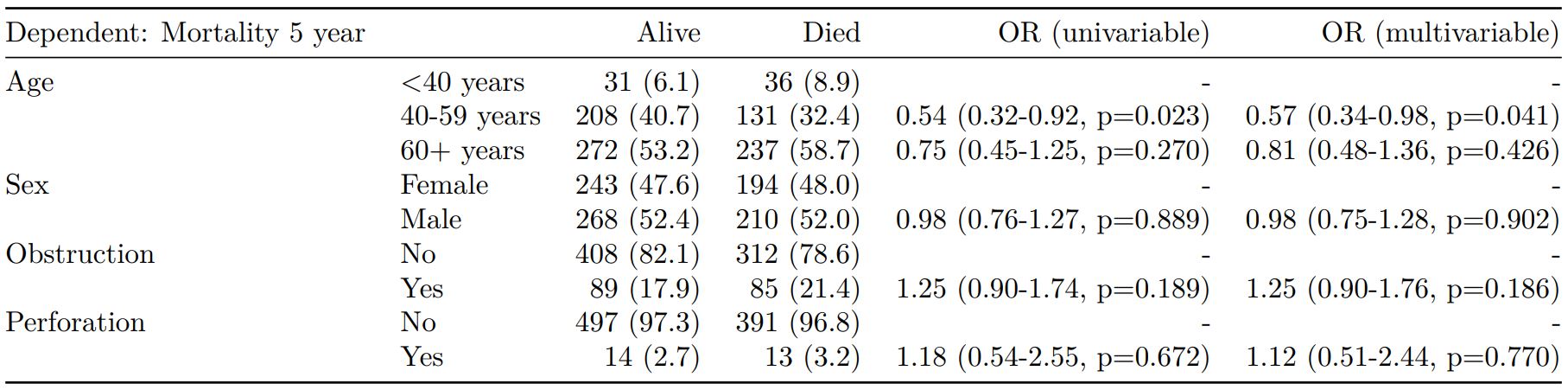
### 2. Summarise regression model results in final table format
The second main feature is the ability to create final tables for linear `lm()`, logistic `glm()`, hierarchical logistic `lme4::glmer()` and Cox proportional hazards `survival::coxph()` regression models.
The `finalfit()` "all-in-one" function takes a single dependent variable with a vector of explanatory variable names (continuous or categorical variables) to produce a final table for publication including summary statistics, univariable and multivariable regression analyses. The first columns are those produced by `summary_factorist()`. The appropriate regression model is chosen on the basis of the dependent variable type and other arguments passed.
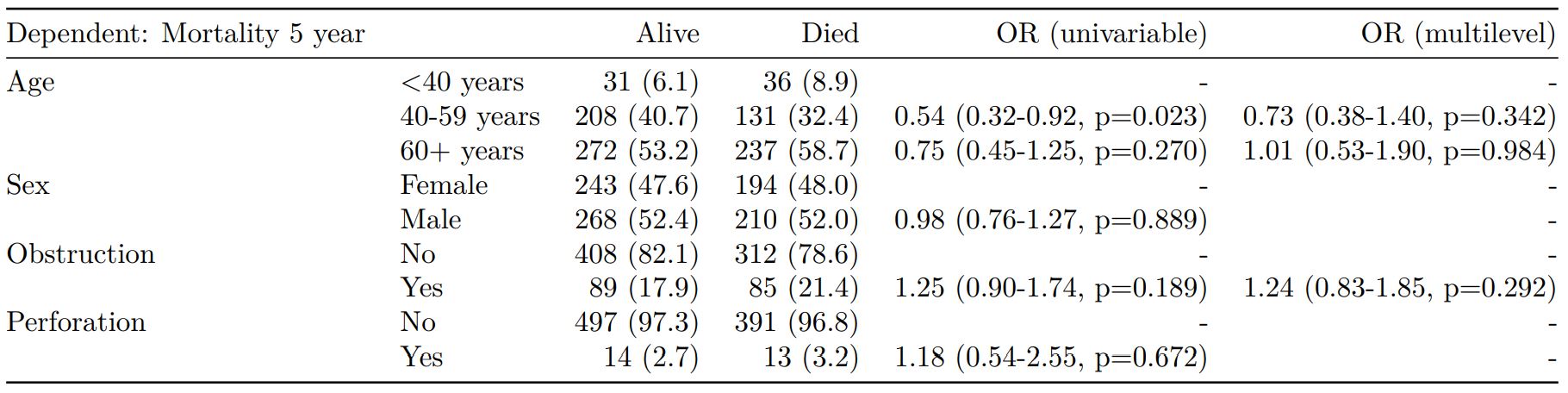
#### Logistic regression: glm()
Of the form: `glm(depdendent ~ explanatory, family="binomial")`
```{r, warning=FALSE, message=FALSE}
explanatory = c("age.factor", "sex.factor", "obstruct.factor", "perfor.factor")
dependent = 'mort_5yr'
colon_s %>%
finalfit(dependent, explanatory) -> t3
knitr::kable(t3, row.names=FALSE, align=c("l", "l", "r", "r", "r", "r"))
```
When exported to PDF:
Tables can be knitted to PDF, Word or html documents. We do this in RStudio from a .Rmd document.
### 2. Summarise regression model results in final table format
The second main feature is the ability to create final tables for linear `lm()`, logistic `glm()`, hierarchical logistic `lme4::glmer()` and Cox proportional hazards `survival::coxph()` regression models.
The `finalfit()` "all-in-one" function takes a single dependent variable with a vector of explanatory variable names (continuous or categorical variables) to produce a final table for publication including summary statistics, univariable and multivariable regression analyses. The first columns are those produced by `summary_factorist()`. The appropriate regression model is chosen on the basis of the dependent variable type and other arguments passed.
#### Logistic regression: glm()
Of the form: `glm(depdendent ~ explanatory, family="binomial")`
```{r, warning=FALSE, message=FALSE}
explanatory = c("age.factor", "sex.factor", "obstruct.factor", "perfor.factor")
dependent = 'mort_5yr'
colon_s %>%
finalfit(dependent, explanatory) -> t3
knitr::kable(t3, row.names=FALSE, align=c("l", "l", "r", "r", "r", "r"))
```
When exported to PDF:
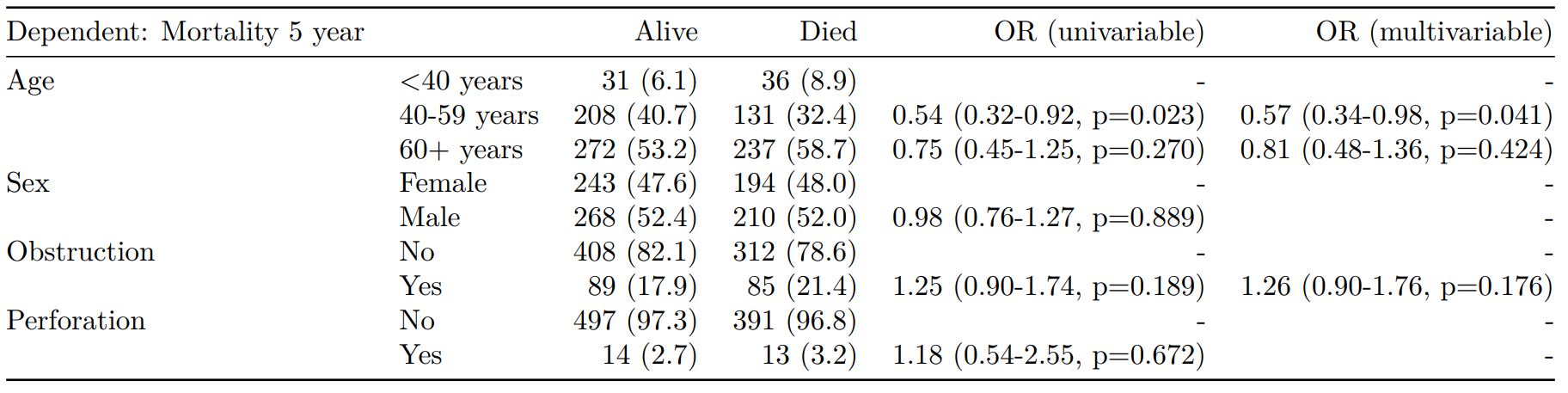
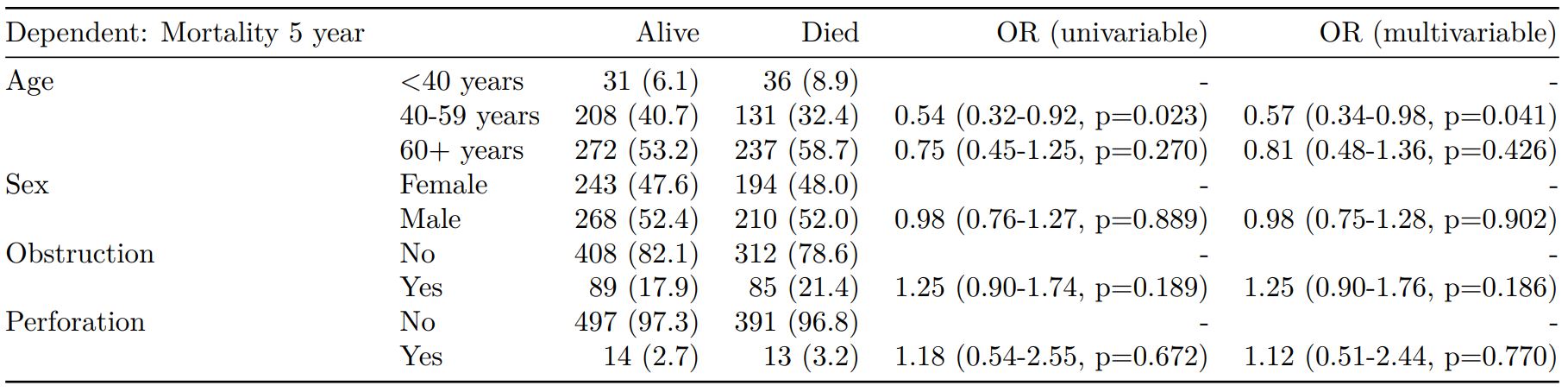
 #### Logistic regression with reduced model: glm()
Where a multivariable model contains a subset of the variables included specified in the full univariable set, this can be specified.
```{r, warning=FALSE, message=FALSE}
explanatory = c("age.factor", "sex.factor", "obstruct.factor", "perfor.factor")
explanatory_multi = c("age.factor", "obstruct.factor")
dependent = 'mort_5yr'
colon_s %>%
finalfit(dependent, explanatory, explanatory_multi) -> t4
knitr::kable(t4, row.names=FALSE, align=c("l", "l", "r", "r", "r", "r"))
```
When exported to PDF:
#### Logistic regression with reduced model: glm()
Where a multivariable model contains a subset of the variables included specified in the full univariable set, this can be specified.
```{r, warning=FALSE, message=FALSE}
explanatory = c("age.factor", "sex.factor", "obstruct.factor", "perfor.factor")
explanatory_multi = c("age.factor", "obstruct.factor")
dependent = 'mort_5yr'
colon_s %>%
finalfit(dependent, explanatory, explanatory_multi) -> t4
knitr::kable(t4, row.names=FALSE, align=c("l", "l", "r", "r", "r", "r"))
```
When exported to PDF:
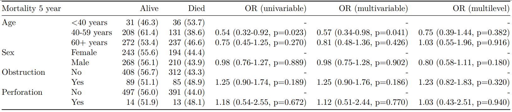
 #### Mixed effects logistic regression: lme4::glmer()
Of the form: `lme4::glmer(dependent ~ explanatory + (1 | random_effect), family="binomial")`
Hierarchical/mixed effects/multilevel logistic regression models can be specified using the argument `random_effect`. At the moment it is just set up for random intercepts (i.e. `(1 | random_effect)`, but in the future I'll adjust this to accommodate random gradients if needed (i.e. `(variable1 | variable2)`.
```{r, warning=FALSE, message=FALSE}
explanatory = c("age.factor", "sex.factor", "obstruct.factor", "perfor.factor")
explanatory_multi = c("age.factor", "obstruct.factor")
random_effect = "hospital"
dependent = 'mort_5yr'
colon_s %>%
finalfit(dependent, explanatory, explanatory_multi, random_effect) -> t5
knitr::kable(t5, row.names=FALSE, align=c("l", "l", "r", "r", "r", "r"))
```
When exported to PDF:
#### Mixed effects logistic regression: lme4::glmer()
Of the form: `lme4::glmer(dependent ~ explanatory + (1 | random_effect), family="binomial")`
Hierarchical/mixed effects/multilevel logistic regression models can be specified using the argument `random_effect`. At the moment it is just set up for random intercepts (i.e. `(1 | random_effect)`, but in the future I'll adjust this to accommodate random gradients if needed (i.e. `(variable1 | variable2)`.
```{r, warning=FALSE, message=FALSE}
explanatory = c("age.factor", "sex.factor", "obstruct.factor", "perfor.factor")
explanatory_multi = c("age.factor", "obstruct.factor")
random_effect = "hospital"
dependent = 'mort_5yr'
colon_s %>%
finalfit(dependent, explanatory, explanatory_multi, random_effect) -> t5
knitr::kable(t5, row.names=FALSE, align=c("l", "l", "r", "r", "r", "r"))
```
When exported to PDF:
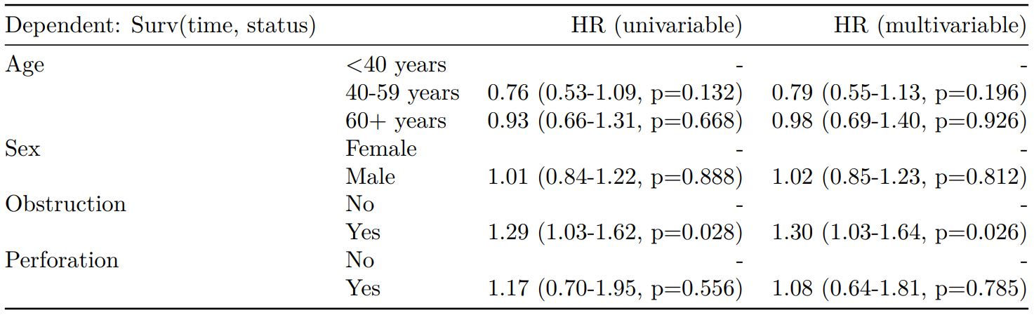
 #### Cox proportional hazards: survival::coxph()
Of the form: `survival::coxph(dependent ~ explanatory)`
```{r, warning=FALSE, message=FALSE}
explanatory = c("age.factor", "sex.factor", "obstruct.factor", "perfor.factor")
dependent = "Surv(time, status)"
colon_s %>%
finalfit(dependent, explanatory) -> t6
knitr::kable(t6, row.names=FALSE, align=c("l", "l", "r", "r", "r", "r"))
```
When exported to PDF:
#### Cox proportional hazards: survival::coxph()
Of the form: `survival::coxph(dependent ~ explanatory)`
```{r, warning=FALSE, message=FALSE}
explanatory = c("age.factor", "sex.factor", "obstruct.factor", "perfor.factor")
dependent = "Surv(time, status)"
colon_s %>%
finalfit(dependent, explanatory) -> t6
knitr::kable(t6, row.names=FALSE, align=c("l", "l", "r", "r", "r", "r"))
```
When exported to PDF:
 #### Add common model metrics to output
`metrics=TRUE` provides common model metrics. The output is a list of two dataframes. Note chunk specification for output below.
```{r, warning=FALSE, message=FALSE}
explanatory = c("age.factor", "sex.factor",
"obstruct.factor", "perfor.factor")
dependent = 'mort_5yr'
colon_s %>%
finalfit(dependent, explanatory, metrics=TRUE) -> t7
knitr::kable(t7[[1]], row.names=FALSE, align=c("l", "l", "r", "r", "r", "r"))
knitr::kable(t7[[2]], row.names=FALSE, col.names="")
```
When exported to PDF:
#### Add common model metrics to output
`metrics=TRUE` provides common model metrics. The output is a list of two dataframes. Note chunk specification for output below.
```{r, warning=FALSE, message=FALSE}
explanatory = c("age.factor", "sex.factor",
"obstruct.factor", "perfor.factor")
dependent = 'mort_5yr'
colon_s %>%
finalfit(dependent, explanatory, metrics=TRUE) -> t7
knitr::kable(t7[[1]], row.names=FALSE, align=c("l", "l", "r", "r", "r", "r"))
knitr::kable(t7[[2]], row.names=FALSE, col.names="")
```
When exported to PDF:
 #### Combine multiple models into single table
Rather than going all-in-one, any number of subset models can be manually added on to a `summary_factorlist()` table using `finalfit_merge()`. This is particularly useful when models take a long-time to run or are complicated.
Note the requirement for `fit_id=TRUE` in `summary_factorlist()`. `fit2df` extracts, condenses, and add metrics to supported models.
```{r, warning=FALSE, message=FALSE}
explanatory = c("age.factor", "sex.factor", "obstruct.factor", "perfor.factor")
explanatory_multi = c("age.factor", "obstruct.factor")
random_effect = "hospital"
dependent = 'mort_5yr'
# Separate tables
colon_s %>%
summary_factorlist(dependent,
explanatory, fit_id=TRUE) -> example.summary
colon_s %>%
glmuni(dependent, explanatory) %>%
fit2df(estimate_suffix=" (univariable)") -> example.univariable
colon_s %>%
glmmulti(dependent, explanatory) %>%
fit2df(estimate_suffix=" (multivariable)") -> example.multivariable
colon_s %>%
glmmixed(dependent, explanatory, random_effect) %>%
fit2df(estimate_suffix=" (multilevel)") -> example.multilevel
# Pipe together
example.summary %>%
finalfit_merge(example.univariable) %>%
finalfit_merge(example.multivariable) %>%
finalfit_merge(example.multilevel, last_merge = TRUE) %>%
dependent_label(colon_s, dependent, prefix="") -> t8 # place dependent variable label
knitr::kable(t8, row.names=FALSE, align=c("l", "l", "r", "r", "r", "r", "r"))
```
When exported to PDF:
#### Combine multiple models into single table
Rather than going all-in-one, any number of subset models can be manually added on to a `summary_factorlist()` table using `finalfit_merge()`. This is particularly useful when models take a long-time to run or are complicated.
Note the requirement for `fit_id=TRUE` in `summary_factorlist()`. `fit2df` extracts, condenses, and add metrics to supported models.
```{r, warning=FALSE, message=FALSE}
explanatory = c("age.factor", "sex.factor", "obstruct.factor", "perfor.factor")
explanatory_multi = c("age.factor", "obstruct.factor")
random_effect = "hospital"
dependent = 'mort_5yr'
# Separate tables
colon_s %>%
summary_factorlist(dependent,
explanatory, fit_id=TRUE) -> example.summary
colon_s %>%
glmuni(dependent, explanatory) %>%
fit2df(estimate_suffix=" (univariable)") -> example.univariable
colon_s %>%
glmmulti(dependent, explanatory) %>%
fit2df(estimate_suffix=" (multivariable)") -> example.multivariable
colon_s %>%
glmmixed(dependent, explanatory, random_effect) %>%
fit2df(estimate_suffix=" (multilevel)") -> example.multilevel
# Pipe together
example.summary %>%
finalfit_merge(example.univariable) %>%
finalfit_merge(example.multivariable) %>%
finalfit_merge(example.multilevel, last_merge = TRUE) %>%
dependent_label(colon_s, dependent, prefix="") -> t8 # place dependent variable label
knitr::kable(t8, row.names=FALSE, align=c("l", "l", "r", "r", "r", "r", "r"))
```
When exported to PDF:
 #### Bayesian logistic regression: with `stan`
Our own particular `rstan` models are supported and will be documented in the future. Broadly, if you are running (hierarchical) logistic regression models in [Stan](https://mc-stan.org/users/interfaces/rstan) with coefficients specified as a vector labelled `beta`, then `fit2df()` will work directly on the `stanfit` object in a similar manner to if it was a `glm` or `glmerMod` object.
### 3. Summarise regression model results in plot
Models can be summarized with odds ratio/hazard ratio plots using `or_plot`, `hr_plot` and `surv_plot`.
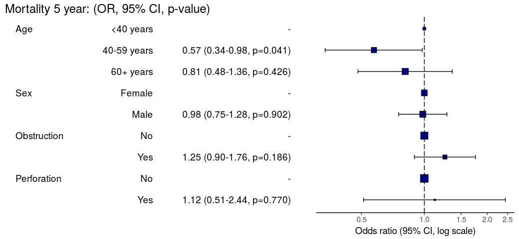
#### OR plot
```{r, eval=FALSE}
explanatory = c("age.factor", "sex.factor", "obstruct.factor", "perfor.factor")
dependent = 'mort_5yr'
colon_s %>%
or_plot(dependent, explanatory)
# Previously fitted models (`glmmulti()` or # `glmmixed()`) can be provided directly to `glmfit`
```
#### Bayesian logistic regression: with `stan`
Our own particular `rstan` models are supported and will be documented in the future. Broadly, if you are running (hierarchical) logistic regression models in [Stan](https://mc-stan.org/users/interfaces/rstan) with coefficients specified as a vector labelled `beta`, then `fit2df()` will work directly on the `stanfit` object in a similar manner to if it was a `glm` or `glmerMod` object.
### 3. Summarise regression model results in plot
Models can be summarized with odds ratio/hazard ratio plots using `or_plot`, `hr_plot` and `surv_plot`.
#### OR plot
```{r, eval=FALSE}
explanatory = c("age.factor", "sex.factor", "obstruct.factor", "perfor.factor")
dependent = 'mort_5yr'
colon_s %>%
or_plot(dependent, explanatory)
# Previously fitted models (`glmmulti()` or # `glmmixed()`) can be provided directly to `glmfit`
```
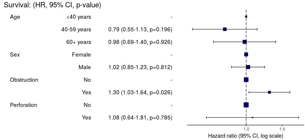
 #### HR plot
```{r, eval=FALSE}
explanatory = c("age.factor", "sex.factor", "obstruct.factor", "perfor.factor")
dependent = "Surv(time, status)"
colon_s %>%
hr_plot(dependent, explanatory, dependent_label = "Survival")
# Previously fitted models (`coxphmulti`) can be provided directly using `coxfit`
```
#### HR plot
```{r, eval=FALSE}
explanatory = c("age.factor", "sex.factor", "obstruct.factor", "perfor.factor")
dependent = "Surv(time, status)"
colon_s %>%
hr_plot(dependent, explanatory, dependent_label = "Survival")
# Previously fitted models (`coxphmulti`) can be provided directly using `coxfit`
```
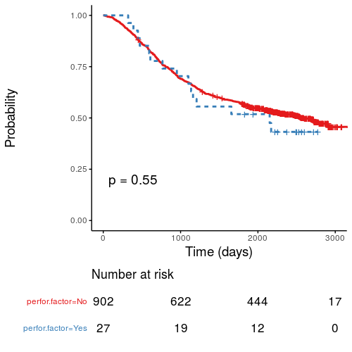
 #### Kaplan-Meier survival plots
KM plots can be produced using the `library(survminer)`
```{r, eval=FALSE}
explanatory = c("perfor.factor")
dependent = "Surv(time, status)"
colon_s %>%
surv_plot(dependent, explanatory,
xlab="Time (days)", pval=TRUE, legend="none")
```
#### Kaplan-Meier survival plots
KM plots can be produced using the `library(survminer)`
```{r, eval=FALSE}
explanatory = c("perfor.factor")
dependent = "Surv(time, status)"
colon_s %>%
surv_plot(dependent, explanatory,
xlab="Time (days)", pval=TRUE, legend="none")
```
 ## Notes
Use `ff_label()` to assign labels to variables for tables and plots.
```{r, eval=FALSE}
colon_s %>%
mutate(
ff_label(age.factor, "Age (years)")
)
```
Export dataframe tables directly or to R Markdown `knitr::kable()`.
Note wrapper `missing_pattern()` is also useful. Wraps `mice::md.pattern`.
```{r, warning=FALSE, message=FALSE}
colon_s %>%
missing_pattern(dependent, explanatory)
```
Development will be on-going, but any input appreciated.
## Notes
Use `ff_label()` to assign labels to variables for tables and plots.
```{r, eval=FALSE}
colon_s %>%
mutate(
ff_label(age.factor, "Age (years)")
)
```
Export dataframe tables directly or to R Markdown `knitr::kable()`.
Note wrapper `missing_pattern()` is also useful. Wraps `mice::md.pattern`.
```{r, warning=FALSE, message=FALSE}
colon_s %>%
missing_pattern(dependent, explanatory)
```
Development will be on-going, but any input appreciated.